Linear Regression With One Varible

Contents

• What is Linear Regression

• Cost Function

• Gradient Descent

What is Linear Regression

Linear regression is a simple and powerful supervised learning technique. The aim of linear regression is to identify the relationship input variable and output variable. The core components in a linear regression are,

1. Continuous input variable
2. Continuous response variable.
3. The assumptions of linear regression being meet.

Here is the example of linear regression for house price prediction. In given example our friend wants to sell hos house with size is 220.

One thing we can do is that to draw a straight line (/) in data and based on that we can tell our friend the price of the house can be 270K $. This problem is called supervised learning algorithm and Regression problem.

 Here is the work of supervised learning algorithm.

 - Learning algorithm starts with training set which contain (m) number of training examples with some input variable (x) and output variable (y). x⁽ⁱ⁾ denotes i ^th training example and y⁽ⁱ⁾ denotes i ^th output example

 - Training set is use to feed data to the learning algorithm. Learning algorithm will create one function called hypothesis (h). This function is relationship between input variable and output variable. It take input variable x and give predicted value y. 

 - How to represent (h) ?

   hθ(x) = θo + θ1x

   h(x) = θo + θ1x

- h(x) = θo + θ1x

- Here h(x) is predicting is a linear function on X and Y is some straight line on X

- This model is call linear regression model

- Model is with one variable or uni-variable linear regression because there is only single input variable

Cost Function

- Cost function is use to figure out that  how to fit the best possible straight line to our data.

- Lets understand cost function and hypothesis calculation with example. Consider bellow training example

X(Input, Independent variable) = 0, 1, 2, 3, 4
Y(Output, Dependent variable) = 0, 1, 2, 3, 4 

- Hypothesis =  h(x) = θo + θ1x

- θi's = Parameter

- We know that how to graph value θo and θ1. With different parameters of θo and θ1 we get different hypothesis function.

- Ex. When θo = 1.5  and  θ1 = 0, The graph looks like

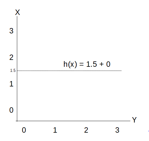
- From this we get h(x) = 1.5

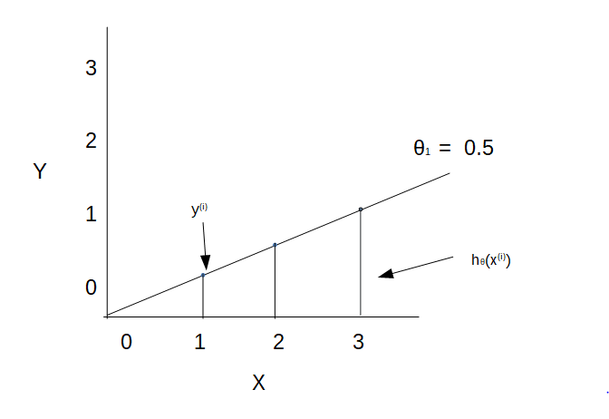
Now θo = 0 and  θ1 = 0.5 

 

Now θo = 1 and  θ1 = 0.5 then,

- In linear regression we have a training set and we have to come up with value for the parameters θo and θ1, so the straight line in data fit well. So how to come with value of θo & θ1 that corresponds to a good fit to the data.

- Solution for that :- Choose  θo, θ1  so that h(x) is close to Y for our training example (x, y). i.e we need to choose θo and θ1  so that our hypothesis function which take input value and predict value is close to Y for our training example, so we can say that the line is good fitted to our data.

- Formula for that  :-  We need to subtract  x⁽ⁱ⁾ (where (i) denotes i ^th training example) with y⁽ⁱ⁾ to get predicted value closest to Y. So,

- Formula
  _m
  Σ( hθ(x⁽ⁱ⁾) - y⁽ⁱ⁾)
  ^{i = 1} 
- Here h(x) = θo + θ1x  ----> Predicted value

- Our goal is to minimize θo and θ1  So we need to divide it with double of number of training example i.e (2 x m). So our formula is now
                                                  m
- minimize (θo, θ1)  = 1/(2m) x Σ( hθ(x⁽ⁱ⁾) - y⁽ⁱ⁾)
                                                  _{i = 1}

- This function is called Cost function or Squared error and denoted by J( θo, θ1). 

 - Cost function intuition

- We need to first define our goal. We have bellow information.

- Hypothesis :  h(x) = θo + θ1x

                                          m

- Cost Function : 1/(2m) x Σ( hθ(x⁽ⁱ⁾) - y⁽ⁱ⁾)

                                        i = 1  

- Goal : minimize J( θo, θ1).

- Now lets compute formula with different values of θ

- When θ1 = 1 then plot looks like

By using given formula
J(θ1) = 1/2m  [(1(1) - 1)² + (1(2) - 2)² + (1(3) - 3)²]

^{J(θ1) = 1/2m [(1-1)2 + (2-2)2 + (3-3)2]}

^{J(θ1) = 1/2m [(0)2 + (0)2 + (0)2]}

^{J(θ1) = 1/2m [0 + 0 + 0]}

J(θ1) = 1/(2(3))  (0)  = (0 / 6)

J(θ1) =0

 - When θ1 = 0.5 then plot looks like

By using given formula
J(θ1) = 1/2m  [(0.5(1) - 1)² + (0.5(2) - 2)² + (0.5(3) - 3)²]

^{J(θ1) = 1/2m [(0.5-1)2 + (1-2)2 + (1.5-3)2]}

^{J(θ1) = 1/2m [(-0.5)2 + (-1)2 + (-1.5)2]}

^{J(θ1) = 1/2m [0.25 + 1 + 2.25]}

J(θ1) = 1/(2(3))  (3.5)  = (3.5 / 6)

J(θ1) = 0.58

 - When θ1 = 0 then plot looks like

By using given formula
J(θ1) = 1/2m  [(0(1) - 1)² + (0(2) - 2)² + (0(3) - 3)²]

^{J(θ1) = 1/2m [(0-1)2 + (0-2)2 + (0-3)2]}

^{J(θ1) = 1/2m [(-1)2 + (-2)2 + (-3)2]}

^{J(θ1) = 1/2m [1 + 4 + 9]}

J(θ1) = 1/(2(3))  (14)  = (14 / 6)

J(θ1) = 2.3

- Now we have some different value of  J(θ1) with θ1. For different different value of  θ1 We get different value of cost function J 

-  θ1 = 1 ---> J(θ1) = 0
-  θ1 = 0.5 ---> J(θ1) =0.58
-  θ1 = 0 ---> J(θ1) = 2.3
  
- Lets plot this value in graph 

   

 - Here we can see that the best fitted value of θ1 = 1. It give us straight line and minimum of  J(θ1) 

 - Objective is to minimize J(θ1) and θ1 = 1 fits the data well and fullfil our objective.

 - By computing this formula with different different value of θ1 = 1then we get different value of  J(θ1). In that case we can also get negative value of  J(θ1).

  - For more understanding please see Quantual Plots.